Automatic Ball-on-Beam Balancer Using Closed-Loop PID Control and Kalman Filtering

ABSTRACT

This paper presents the design and implementation of an Automatic Ball-on-Beam Balancer using closed-loop control on a Tiva C TM4C123GH6PM ARM Cortex-M4 microcontroller. A Sharp GP2Y0A41SK0F infrared sensor provides continuous ball position feedback. A 2-state Kalman Filter suppresses sensor noise while simultaneously estimating ball velocity. A discrete-time PID controller with Exponential Moving Average (EMA) derivative smoothing drives an SG90 servo motor to tilt a 350mm 3D-printed beam. The control loop executes at 50Hz via a hardware Timer ISR with no operating system.

All PID gains are tunable at runtime over UART without recompilation. The system achieves stable ball positioning with sub-centimeter steady-state error, demonstrating practical real-time embedded control.
Keywords: Ball-on-Beam, PID Control, Kalman Filter, Tiva C, ARM Cortex-M4, Embedded Systems, Sharp IR Sensor, Servo Motor.

I.INTRODUCTION

The ball-on-beam system is a canonical benchmark in control systems engineering. It is inherently unstable: a ball placed anywhere on the beam will roll off within seconds without ac-tive feedback. This property makes it ideal for validating PID controllers, state observers, and sensor fusion algorithms un-der realistic dynamics.

Unlike simulation-based demonstrations, this project implements the complete control system in hardware on a single microcontroller with no external processors, no operating system, and no cloud connectivity. All sensing, filtering, computation, and actuation occur within a 20 ms hardware interrupt service routine (ISR).

The design integrates four theoretical disciplines analog sensor characterisation, Kalman state estimation, discrete-time PID theory, and PWM-based servo actuation into a unified 50 Hz real-time control loop, demonstrating the full embedded systems design flow from mathematical model to physical hardware.

II.SYSTEM OVERVIEW

The system comprises four subsystems: sensing, filtering, computation, and actuation. These are orchestrated by a 50 Hz hardware timer ISR on the Tiva C microcontroller.

2.1 Hardware Architecture

The system is built around the Tiva C TM4C123GH6PM ARM Cortex-M4 microcontroller running at 80 MHz. A Sharp GP2Y0A41SK0F infrared sensor provides analog ball position feedback via the on-chip 12-bit ADC. An SG90 servo motor actuates the beam tilt through a double-clevis pushrod link-age, driven by the microcontroller’s hardware PWM module. A USB-UART bridge enables live gain tuning and telemetry streaming at 115200 baud. Table 2.1 summarises all hardware components and their interfaces.

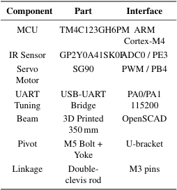
Table 1: Hardware Components

2.2 Control Loop Pipeline

Every 20 ms, the following five-step pipeline executes inside the Timer0A Handler hardware ISR:

1. SENSE — ADC0 samples Sharp IR (12-bit, AIN0)
2. FILTER — 2-state Kalman estimates position and velocity
3. THINK — PID with EMA derivative computes correction
4. ACT — PWM register updated to tilt beam via servo
5. STREAM — Telemetry packet sent via UART at 10 Hz 1 illustrates the complete 50 Hz control loop as executed inside Timer0A Handler.

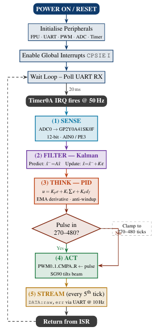
Figure 1: Complete 50Hz control loop. Boot initialises peripherals; the wait loop polls UART for live gain commands. Every 20ms, Timer0A fires the ISR which executes five colour-coded stages: Sense, Filter (Kalman), Think (PID), Act (PWM), and Stream (UART)

III.SENSOR CHARACTERISATION

3.1 Sharp GP2Y0A41SK0F

The Sharp GP2Y0A41SK0F is an analog infrared distance sensor operating on the triangulation principle. An infrared LED illuminates the target; a Position Sensitive Device (PSD) detects the reflected beam angle, which varies with distance. The sensor outputs an analog voltage following an inverse relationship with distance over its 4–30 cm measurement range, matching the effective ball travel range on the 350 mm beam.

The sensor was selected over the longer-range GP2Y0A21YK0F (10–80 cm) because its 4 cm minimum distance prevents the voltage curve inversion problem: theGP2Y0A21 produces ambiguous (rising) output below 10 cm, causing the PID controller to receive false position data when the ball approaches the sensor end. The GP2Y0A41 maintains monotonically decreasing output throughout the beam’s usable range.

3.2 Distance–Voltage Model

The sensor output voltage V is related to distance d by the empirical inverse model:

where ADC_raw is the 12-bit ADC reading (0–4095) corresponding to the 0–3.3 V output range, and k = 14336 is an empirical constant calibrated for 3.3 V supply. The control loop operates entirely in ADC count space; centimetre conversion is performed only for display purposes.

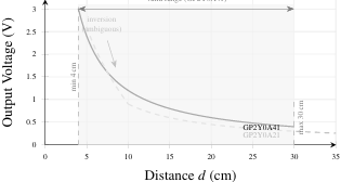Figure 2: Sharp IR sensor output voltage vs. distance. The GP2Y0A41SK0F (solid) maintains monotonically decreasing output across the full 4–30 cm beam range. The GP2Y0A21YK0F (dashed) inverts below 10 cm, producing ambiguous readings that would corrupt the PID derivative term

3.3 ADC Configuration

ADC0 is configured in single-sample mode using Sequencer 3 (SS3) on channel AIN0 (PE3). The ADC is triggered by software from within the Timer ISR and polled for completion. This software-triggered approach ensures exact synchronisation between the ADC sample and the control computation with deterministic 12-bit precision.

IV.KALMAN FILTER THEORY

Raw ADC readings exhibit approximately ±20–40 ADC count noise at static positions, caused by IR ambient interference, quantisation, and sensor electronics noise. Feeding this noise directly into the PID derivative term amplifies it by a factor of K_d per timestep, causing visible servo jitter. A 2-state Kalman Filter optimally suppresses this noise while simultaneously estimating ball velocity as a by-product of state estimation.

4.1 The Core Problem — Sensor Noise

To illustrate why raw sensor data is dangerous for PID control, consider the ball stationary at a true position of 175 mm. Four successive IR sensor readings might be: 181 mm, 169 mm, 178 mm, 172 mm. If the PID receives these directly, the derivative term K_d sees a rate of change of ±12 mm per sample a completely fictitious velocity that drives the servo to twitch violently even though the ball is not moving.

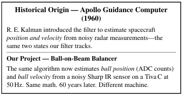
Figure 3: The Kalman Filter was first applied to the Apollo lunar guidance computer to estimate spacecraft trajectory from noisy radar. This project applies the identical two-state framework to estimate ball position and velocity from a Sharp IR sensor

4.2 The Two-Expert Intuition
The Kalman Filter can be understood as two competing estimators reconciled at every timestep:
• Predictor (Physics Model): Uses the dynamic model and previous state estimate to predict the current position the a priori estimate xˆ−.
• Corrector (Sensor Measurement): Provides a direct but noisy observation yk of the true position the measurement update.

The filter blends both estimates in proportion to their respective uncertainties. The Kalman gain K determines this weighting automatically adjusted every timestep to minimise the posterior estimation error covariance. This is what makes Kalman optimal for stochastic systems: processes with inherent randomness where future state probabilistically de-pends on current conditions.

4.3 State Observer Block Diagram
Fig. 4 shows the state observer architecture from which the Kalman Filter is derived. The physical plant and the mathematical model run in parallel; the observer corrects its estimate by feeding back the difference between the real output y and its predicted output ˆy, scaled by gain K.

4.4 Observer Error Convergence

Let the observation error be e_obs = x − xˆ. Subtracting the ob-server dynamics from the plant dynamics:

e˙_obs = (A − KC) e_obs     (2)

This has the solution:

eobs(t) = e(A−KC)t eobs(0)     (3)

Key result: if (A − KC) < 0, then e_obs → 0 as t → ∞, meaning xˆ → x. The Kalman Filter automatically computes the optimal K at every timestep by minimising the expected squared estimation error, guaranteeing convergence for our system.

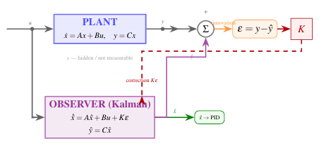
Figure 4: State observer architecture (from lecture notes). The Plant (physical system) and Observer (Kalman mathematical model) run in parallel. The innovation ε = y− ˆy scaled by gain K corrects the observer’s estimate every timestep. Output ˆx feeds the PID controller

The filter models the ball with two state variables: position x (ADC counts) and velocity v (ADC counts per second). The discrete-time state transition model at timestep ∆t = 0.02 s is:

x_k = x_k−1 + v_k−1 ∆t,   v_k = v_k−1                    (4)

The measurement model assumes direct observation of position with additive Gaussian noise: y_k = x_k + ν, ν ∼ N (0, R).

4.5 Predict Step

Before examining the sensor reading, the filter extrapolates its state estimate using the physical model. The state estimate and its associated error covariance matrix P evolve as:

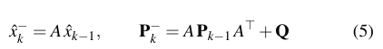
where Q is the process noise covariance matrix, parameterised by Q_pos = 0.01 and Q_vel = 0.01.

4.6 Update Step

After the ADC sample is obtained, the filter computes the optimal Kalman gain K and corrects the state estimate:

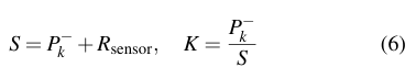
where R_sensor = 15.0 is the sensor noise covariance. The in-novation term (y_k − xˆ⁻) represents the discrepancy between measured and predicted position.

4.7 Covariance Matrix Integrity
A critical implementation requirement: the covariance update equations for P10 and P11 must use the pre-update values of P00 and P01. Without saving these before modification, sequential register updates corrupt the covariance matrix, causing P to diverge over time. Divergence causes the Kalman gain to collapse, the filter to produce stale estimates, and the servo to lock at an incorrect position. Saving Pold and Pold before the update step is the standard fix absent in most student-level implementations.

4.8 Velocity Estimation

The velocity state v_est is never directly measured it is inferred from successive position observations through the Kalman up-date equations. This provides a smooth, noise-filtered velocity estimate that would otherwise require noisy finite-difference differentiation of successive ADC readings.

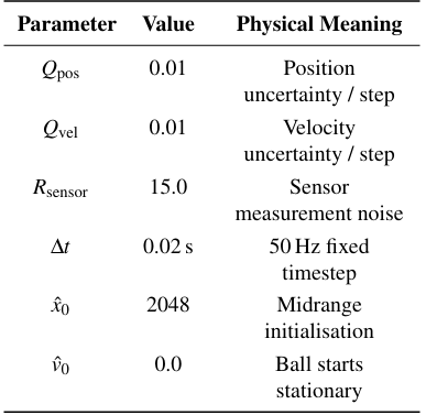
Table 2: Kalman Filter Parameters

V.PID CONTROLLER THEORY
A discrete-time PID controller computes the servo pulse width correction from the filtered position error:

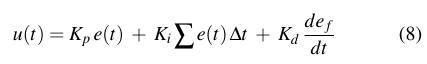
where e(t) = Target ADC − xˆ_filtered is the signed error in ADC counts, and de_f /dt is the EMA-smoothed derivative.

5.1 Proportional Term

The proportional term K_pe provides immediate corrective force proportional to current error and is the dominant restoring term for large deviations. Too large a K_p causes overshoot and oscillation; too small gives a sluggish response. The gain K_p = 0.12 was determined using the Ziegler–Nichols ultimate gain method. With K_i and K_d set to zero, K_p is raised from zero until the closed-loop output exhibits sustained constant amplitude oscillations the ultimate gain K_u. The proportional gain is then set to approximately 60% of K_u, which places the system response below the oscillation boundary with adequate stability margin.  In this project, K_u ≈ 0.20 was identified experimentally, yielding the starting value K_p = 0.12. This was subsequently verified and fine-tuned via live UART commands while the ball was actively balancing.

5.2 Integral Term

The integral term K_i ∑ e accumulates error over time and eliminates steady-state offset caused by gravity-induced bias and mechanical asymmetry. Anti-windup clamping limits the accumulator to ±1000 ADC counts, preventing integrator saturation during large transients. The accumulator resets to zero on every setpoint command.

5.3 Derivative Term with EMA Smoothing

The derivative term predicts future error by measuring error rate of change. In practice, discrete differentiation of noisy ADC readings amplifies high-frequency noise by a factor proportional to the sampling rate, causing severe servo jitter.

An Exponential Moving Average (EMA) filter is applied to the raw derivative before multiplication by K_d. The EMA is a first-order IIR filter:

d _f [k] = α e[k] − e[k−1] + (1 − α) d _f [k−1]         (9)

where α = 0.15 is the smoothing coefficient. A low α provides heavy smoothing (slow response, minimal jitter); high α follows the derivative more closely (fast response, more jitter).

5.4 Servo Actuation Limits

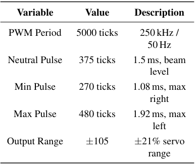
Table 3: PWM Servo Parameters

5.5 Live UART Tuning

All PID gains and the setpoint are modifiable at runtime via UART at 115200 baud. The control loop continues uninterrupted during command reception, enabling iterative in-situ gain tuning while the ball is actively balancing.

VI.STEP RESPONSE ANALYSIS

The closed-loop step response follows a classic second-order profile, consistent with the system’s two dominant poles one from the mechanical integrator (force creates acceleration, not velocity) and one from the PID integral action.

6.1 Rise Phase

Immediately after a setpoint change, the proportional term dominates: the large error drives the servo to near-maximum tilt, causing the ball to accelerate rapidly toward the target. The derivative term begins contributing as velocity builds, applying a braking effect that softens the approach.

6.2 Overshoot and Undershoot

The ball’s inertia carries it past the setpoint despite derivative braking. At peak overshoot, the error reverses sign. The proportional term now acts as a restoring force in the opposite direction while the derivative term, detecting rapid error change, applies additional correction. This produces the undershoot phase as the ball reverses direction.

6.3 Settling

Successive oscillations decay exponentially as energy dissipates through servo actuation and beam friction. The integral term eliminates residual steady-state error. Well-tuned gains produce settling within 2–3 half-oscillations, consistent with a mildly underdamped second-order response.

6.4 Gain Tuning Procedure

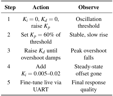
Table 4: Step-by-Step Gain Tuning Procedure

VII.RESULTS

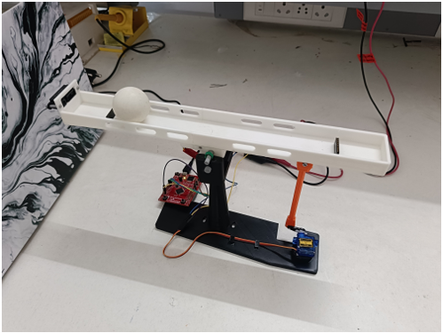
Figure 5: Complete Ball-on-Beam Balancer SG90 servo with double-clevis pushrod, Sharp GP2Y0A41SK0F IR sensor, and 3D printed beam on centre pivot

7.1 Performance Summary

The system achieves stable ball positioning at the commanded setpoint with a measured steady-state error of less than ±1 cm, consistent with sensor quantisation limits (approximately 0.3 cm per ADC count at 22 cm). Disturbance rejection is demonstrated by manually displacing the ball: the system recovers to setpoint within approximately 2–3 seconds. The Kalman filter reduces visible servo jitter from ±3–5 ADC counts (raw) to below ±1 ADC count at static positions. The UART tuning interface reduces iterative gain adjustment from minutes (reflash cycle) to seconds (live command).

VIII.CONCLUSION

A fully functional closed-loop Ball-on-Beam Balancer was successfully designed and implemented on the Tiva C TM4C123GH6PM ARM Cortex-M4 microcontroller. The system integrates 2-state Kalman filtering for sensor noise rejection, discrete-time PID control with EMA derivative smoothing for stable servo actuation, and inverse-model IR sensor characterisation into a unified 50 Hz real-time control loop with no operating system.

The project achieves its primary objective: balancing a ball at a commanded position on an inherently unstable platform, with measurable disturbance rejection and sub-centimetre steady-state error. Future work includes physical button set-point switching, WS2812B RGB LED error visualisation, and an Edge-AI gesture-based setpoint controller using TinyML on an Arduino Nano 33 BLE.

REFERENCES

• Texas Instruments, “Tiva C Series TM4C123GH6PM Microcontroller Data Sheet,” SPMS376E, 2014.
• Sharp Corporation, “GP2Y0A41SK0F Distance Measuring Sensor Data Sheet,” 2006.
• C. Dorf and R. H. Bishop, Modern Control Systems, 13th ed. Pearson, 2017.
• E. Kalman, “A new approach to linear filtering and prediction problems,” ASME Journal of Basic Engineering, vol. 82, pp. 35–45, 1960.
• Welch and G. Bishop, “An introduction to the Kalman filter,” University of North Carolina TR 95-041, 2006.
• Ogata, Discrete-Time Control Systems, 2nd ed. Prentice Hall, 1995. K. J. A˚ stro¨m and T. Ha¨gglund, PID Controllers: Theory, Design, and Tuning, 2nd ed. ISA Press, 1995.