I.INTRODUCTION
1.1 Project Motivation:
Scientific calculators have been an essential tool for students, engineers, and scientists for decades. The implementation of a scientific calculator on a microcontroller platform provides an excellent opportunity to understand both the mathematical algorithms and embedded systems principles. By avoiding the use of floating-point libraries, this project demonstrates efficient fixed-point arithmetic implementation, which is particularly valuable in resource-constrained environments.
This project was inspired by the need for a customizable scientific calculator that could be tailored to specific requirements while maintaining high performance on limited hardware. The implementation demonstrates how complex mathematical operations can be efficiently performed without relying on built-in floating-point units, making it suitable for deployment on a wider range of microcontrollers.
1.2 System Overview:
The calculator system consists of:
• A microcontroller (TIVA C series TM4C123GH6PM)
• Touch LCD display module (Kentec QVGA touch screen)
• UART interface for communication with external devices
• Software components implementing various mathematical functions
The system architecture follows a modular approach where different mathematical operations are implemented as separate modules, which are integrated into a cohesive user interface via the touchscreen display. The UART interface provides an additional method of interaction, allowing the calculator to be controlled remotely or to export calculation results to other systems.
II. Hardware Architecture:
2.1 Microcontroller:
The system uses a TIVA C series TM4C123GH6PM microcontroller, which provides:
• 80 MHz ARM Cortex-M4F CPU
• 256 KB Flash memory
• 32 KB SRAM
• Extensive peripheral set including GPIO, SPI, and UART
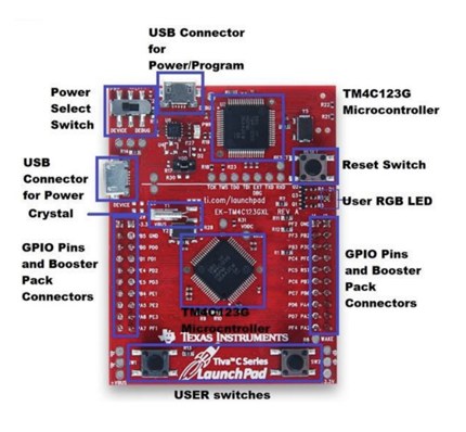
Figure 1: TIVA C Series Launchpad Board
2.2 LCD Touchscreen Interface:
The LCD touchscreen module used is the Kentec QVGA display with touch capability, featuring a resolution of 320×240 pixels and 16-bit color depth. The touch interface uses resistive technology, providing accurate position detection for user input.
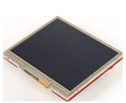
Figure 2: Kentec QVGA Touch Screen Module
Integration with the microcontroller requires:
• SPI communication for display data transfer
• GPIO interfacing for control signals
• ADC channels for touch position detection
• Initialization of the SSD2119 controller for display configuration
The display driver implementation follows a layered approach:
1. Low-level hardware interface (SPI and GPIO control)
2. Display controller commands (initialization, pixel addressing)
3. Graphics primitives (lines, rectangles, text rendering)
4. UI components (buttons, text fields, graphs)
2.3 UART Communication:
The UART interface is implemented using the microcontroller’s built-in UART module. This interface allows:
• Communication with a PC for data logging
• Remote control of calculator functions
• Firmware updates
The UART is configured with standard parameters (115200 baud rate, 8 data bits, no parity, 1 stop
bit) and interfaced directly with the microcontroller’s GPIO pins. The implementation includes:
• Interrupt-driven reception to minimize CPU overhead
• Circular buffers for efficient data handling
• Command parser for interpreting incoming commands
• Formatted output for calculation results
III. Software Architecture:
3.1 Code Organization:
The software follows a hierarchical structure with clearly defined modules for different aspects of the calculator’s functionality:
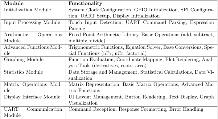
Each module is implemented as a separate C file with a corresponding header, providing clear interfaces between components and facilitating code maintenance and testing.
3.2 Fixed-Point Arithmetic Implementation:
Without the use of a floating-point library, all operations are implemented using fixed-point arithmetic. Numbers are represented as scaled integers, with the scale factor determining the precision. Our implementation uses a 32-bit signed integer (int32 t) to represent fixed-point numbers, with 16 bits allocated for the integer part and 16 bits for the fractional part. This provides a range of approximately ±32,768 with a precision of about 1.5 × 10.
IV. User Interface Design:
4.1 Main Calculator Panel:
The main calculator panel provides access to basic arithmetic operations, memory functions, and navigation to specialized panels. It features a large display area for input and results, along with a numeric keypad and operation buttons.
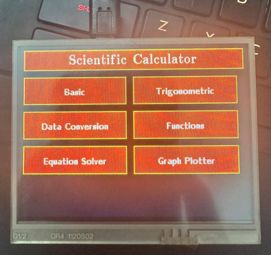
Figure 3: Main Calculator Panel
The main panel includes:
• Numeric keypad (0-9, decimal point)
• Basic operation buttons (+,-, ×, ÷)
• Parentheses and memory function buttons
• Clear and delete buttons
• Navigation buttons to specialized panels
4.2 Scientific Functions Panel:
The scientific functions panel provides access to advanced mathematical operations such as trigonometric, logarithmic, and exponential functions.
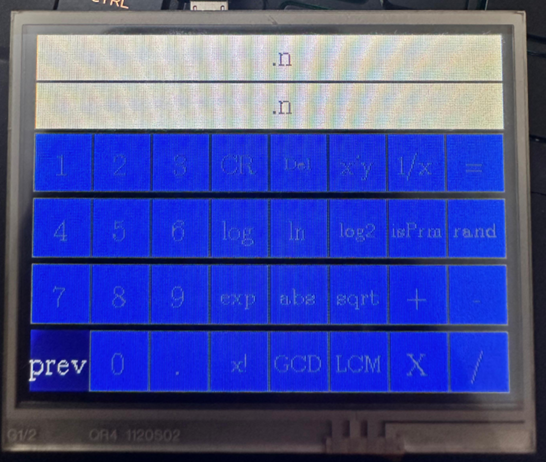
Figure 4: Scientific Functions Panel
This panel includes:
• Trigonometric functions (sin, cos, tan) and their inverses
• Logarithmic functions (log, ln)
• Exponential functions (exp, x²)
• Special functions (nPr, nCr, factorial)
• Constants (, e)
4.3 Equation Solver Panel:
The equation solver panel allows users to solve polynomial equations up to the 3rd degree.
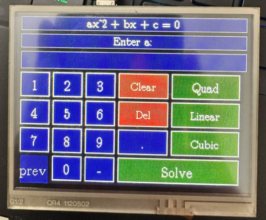
Figure 5: Equation Solver Panel
This panel includes:
• Degree selection (1st, 2nd, 3rd)
• Coefficient input fields
• Solve button
• Results display area
4.4 Base Conversion Panel:
The base conversion panel allows users to convert between different number systems.
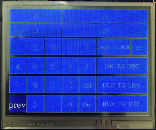
Figure 6: Base Conversion Panel
This panel includes:
• Input field for the number to convert
• Base selection for input (Decimal, Binary, Octal, Hexadecimal)
• Convert button
• Results display in all four bases
4.5 Graph Plotting Panel:
The graph plotting panel allows users to visualize mathematical functions and analyze their properties.
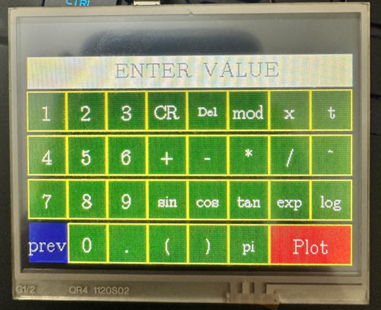
Figure 7: Graph Plotting Panel
This panel includes:
• Function input field
• Range settings for x and y axes
• Graph display area with grid
• Analysis tools (derivatives, zeros, area)
• Zoom and pan controls
4.6 Statistics Panel:
The statistics panel allows users to input data and perform statistical analyses.
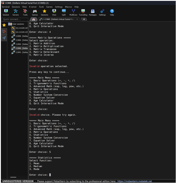
Figure 8: Statistics Panel
This panel includes:
• Data input area
• Basic statistics display (mean, median, mode)
• Standard deviation and variance
• Linear regression analysis
• Data visualization (histogram, scatter plot)
4.7 Matrix Operations Panel:
The matrix operations panel allows users to perform matrix calculations.
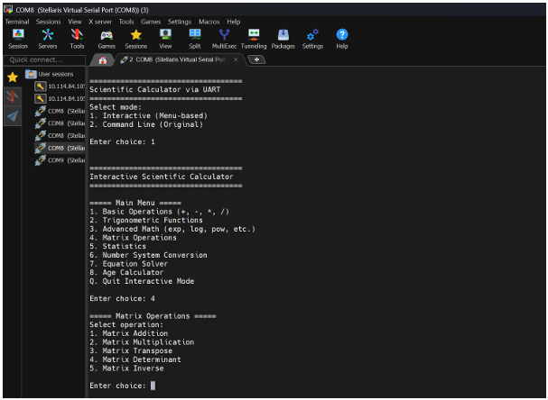
Figure 9: Matrix Operations Panel
This panel includes:
• Matrix dimension selection
• Matrix element input
• Operation selection (addition, subtraction, multiplication, determinant, inverse)
• Result display
V. Implementation of Mathematical Functions:
5.1 Basic Arithmetic Operations:
The fundamental arithmetic operations (addition, subtraction, multiplication, and division) are implemented using the fixed-point arithmetic library. Additional considerations include:
• Overflow detection and handling
• Division by zero prevention
• Rounding strategies for improved accuracy
The expression parser converts infix notation (the standard mathematical notation) to Reverse Polish Notation (RPN) using the Shunting-Yard algorithm, which simplifies the evaluation process. The parser handles operator precedence, parentheses, and function calls.
5.2 Trigonometric Functions:
Trigonometric functions are implemented using Taylor series approximations. For improved performance, the CORDIC (COordinate Rotation DIgital Computer) algorithm is also implemented as an alternative method, particularly well-suited for fixed-point arithmetic.
The implementation includes:
• Sine, cosine, and tangent functions
• Inverse trigonometric functions
• Angle normalization to appropriate ranges
• Degree/radian conversion
5.3 Equation Solver:
The equation solver supports polynomial equations up to 3rd degree. Different algorithms are used based on the degree:
5.3.1 Linear Equations (1st degree)
For linear equations of the form ax + b = 0, the solution is directly computed as x = −b/a.
5.3.2 Quadratic Equations (2nd degree)
For quadratic equations of the form ax2 + bx + c = 0, the quadratic formula is used: x = −b±√a
Special handling is required for the discriminant to determine the number and type of roots.
5.3.3 Cubic Equations (3rd degree)
For cubic equations of the form ax3 + bx2 + cx + d = 0, Cardano’s method is implemented for exact solutions. Additionally, a numerical approach using the Newton-Raphson method is provided as a fallback for cases where Cardano’s method is numerically unstable.
5.4 Base Conversions:
Base conversion functionality allows users to convert between decimal, binary, octal, and hexadecimal number systems. The implementation includes:
• Decimal to binary conversion
• Decimal to octal conversion
• Decimal to hexadecimal conversion
• Binary to decimal conversion
• Octal to decimal conversion
• Hexadecimal to decimal conversion
• Direct conversion between any two bases
5.5 Special Functions:
Special functions such as factorial, combinations (nCr), and permutations (nPr) are implemented with optimizations to prevent overflow and improve performance:
• Factorial calculation with range limiting
• Combination calculation using the multiplicative formula
• Permutation calculation with optimization for large values
• Error handling for invalid inputs
Recent Comments